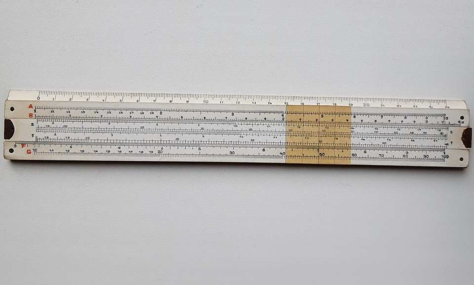
The Slide Rule: An Ancestor of Modern Computing Devices

The slide rule, also called a calculating rule, is a versatile calculating instrument for several mathematical operations: multiplication and division, raising numbers to powers, usually squares and cubes, extracting square and cube roots, finding logarithms and antilogarithms, calculating trigonometric functions, and other operations.

Early in the seventeenth century, the English astronomer Edmund Gunter proposed an idea close to the slide rule’s design. He suggested marking a logarithmic scale on a ruler and using two pairs of compasses to perform addition and subtraction of logarithms.

William Oughtred (1574–1660), credited with the first slide rule, published a version differing little from the modern instrument in his Circles of Proportion (1622). His first rule was circular, but a description of a rectangular rule, attributed to Oughtred, was published in 1633.

William Oughtred (1574–1660), English mathematician and inventor of the slide rule (1622) · Source

Later improvements included a second movable rule, the “slide”, introduced by Robert Bissaker in 1654. The cursor appeared in the mid-nineteenth century, with Victor-Amédée Mannheim.

Operating principle and construction

Before pocket calculators, the slide rule was an indispensable engineering aid. Its calculations were accurate to 3-4 significant figures.

Unlike an ordinary ruler, it has several logarithmic scales, on which each mark a lies at a distance from the scale’s origin proportional to lg a.

Its operation rests on replacing multiplication and division by addition and subtraction of logarithms:

lg (ab) = lg a + lg b
lg (a/b) = lg a − lg b

The simplest slide rule consists of two logarithmic scales that can move relative to each other.

Slide rules came in different shapes and sizes. A standard rule was 30 cm long, convenient for geometric work on A4 paper. Its logarithmic scales were 25 cm long, usually labelled at their ends. Smaller rules with 12.5 cm scales were less common. For secondary-school calculation work, a general-purpose rule with 10 scales was preferred.

A standard rectangular slide rule consists of three parts:

A body with a longitudinal groove.
A cursor: a metal frame with glass bearing lines, called hairlines or indices.
A slide that moves along the body and can also be removed and reinserted with its reverse side facing up.

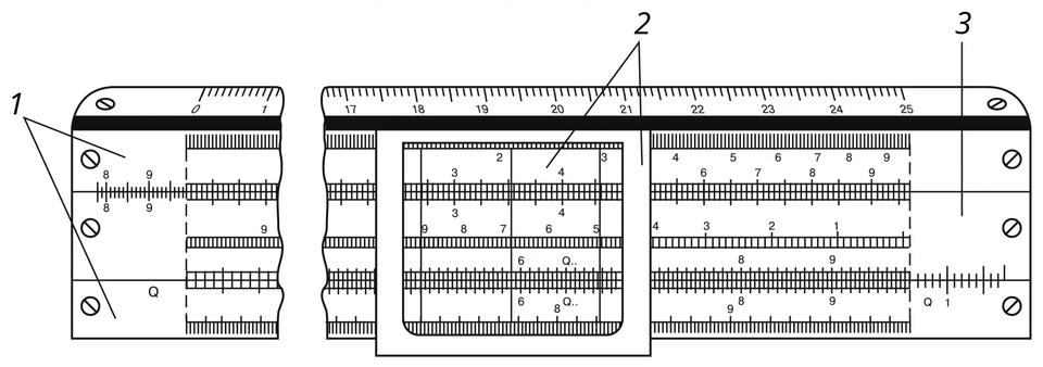
Parts of a slide rule: 1, body; 2, cursor; 3, slide · Source

The front of the body has four scales:

The logarithmic K scale at the top, called the cube scale.
The logarithmic A scale below it, along the upper edge of the groove, called the square scale.
The D scale below that, along the lower edge of the groove, called the main scale.
The uniform L scale along the body’s lower edge, divided into half-millimetres and called the logarithmic mantissa scale, used to find logarithms and antilogarithms.

The front of the slide carries B and C scales, identical to A and D respectively. Between B and C is the R scale, called the “reciprocal scale”, an inverted C scale.

The reverse of the slide carries trigonometric scales.

Slide-rule scales: K, cube scale; A, square scale; D, main scale; L, logarithmic mantissa scale; B and C, identical to A and D respectively; R, reciprocal scale, an inverted C scale · Source

The cursor’s indices help locate the mark on one scale opposite a particular mark on another.

Reference material useful to engineers was printed on the back of the body, while centimetre and millimetre ruler graduations ran along its narrow edges.

Circular slide rules, or logarithmic circles, were also manufactured. Their advantage was compactness.

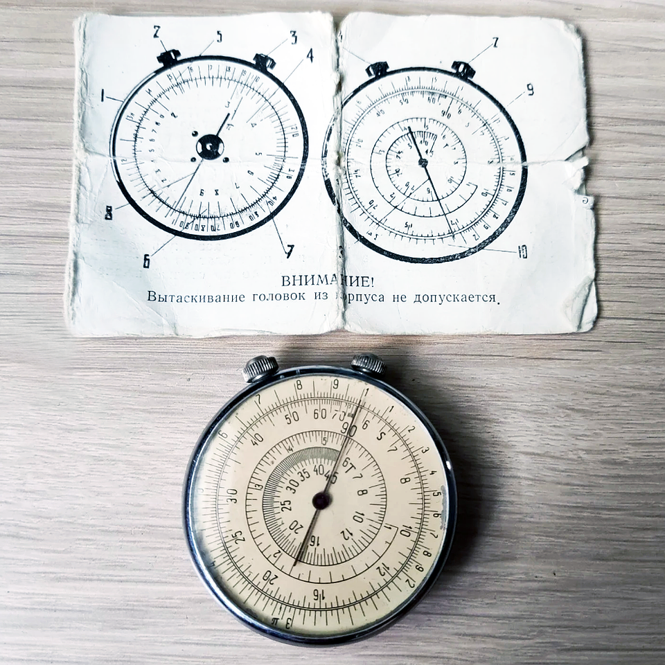
A circular slide rule has two dials. The front has a movable dial with two scales: the main B scale and the C scale of squares.

The reverse has a fixed dial with three scales: a main scale and two trigonometric scales, S for sines and T for tangents. Knobs rotate the movable dial and the hands.

Calculations

To multiply two numbers, align the beginning or end of the movable scale with the first factor on the fixed scale, then locate the second factor on the movable scale. Opposite it, on the fixed scale, is the product.

To divide, locate the divisor on the movable scale and align it with the dividend on the fixed scale. The beginning or end of the movable scale indicates the result.

The slide rule gives only the number’s mantissa; its order of magnitude is worked out mentally.

Other operations use the cursor and additional scales.

Despite its simplicity, a slide rule can perform quite complicated calculations. Manuals with worked practical examples were once published for this purpose. Slide rules were widely used for engineering calculations until around the early 1980s.

A standard calculating rule permits specialized calculations such as:

Solving certain cases of oblique triangles.
Solving right triangles.
Converting Cartesian coordinates to polar coordinates and back.
Calculations with complex numbers.
Converting degrees to radians and back.
Calculating a circle’s circumference and area.
Calculating a cube’s surface area and volume.
Calculating the surface areas and volumes of solids of revolution.

P. S. From the author: “I attended secondary school in Begishevo in 1965–1967. We practised extensively with both slide rules and logarithm tables. I remember our mathematics teacher, Yabbar Subkhanovich Valeyev, even organizing competitions among the pupils for rapid calculation with a slide rule.”

Operating principle and construction

Calculations

Further reading